Query Optimization¶

Updating Statistics¶

With the UPDATE STATISTICS ON statement, you can generate internal statistics used by the query processor. Such statistics allow the database system to perform query optimization more efficiently.

UPDATE STATISTICS ON { table_spec [ {, table_spec } ] | ALL CLASSES | CATALOG CLASSES } [ ; ]

table_spec ::=
single_table_spec
| ( single_table_spec [ {, single_table_spec } ] )

single_table_spec ::=
[ ONLY ] table_name
| ALL table_name [ ( EXCEPT table_name ) ]

• ALL CLASSES : If the ALL CLASSES keyword is specified, the statistics on all the tables existing in the database are updated.

When starting and ending an update of statistics information, NOTIFICATION message is written on the server error log. You can check the updating term of statistics information by these two messages.

Time: 05/07/13 15:06:25.052 - NOTIFICATION *** file ../../src/storage/statistics_sr.c, line 123  CODE = -1114 Tran = 1, CLIENT = testhost:csql(21060), EID = 4
Started to update statistics (class "code", oid : 0|522|3).

Time: 05/07/13 15:06:25.053 - NOTIFICATION *** file ../../src/storage/statistics_sr.c, line 330  CODE = -1115 Tran = 1, CLIENT = testhost:csql(21060), EID = 5
Finished to update statistics (class "code", oid : 0|522|3, error code : 0).

Checking Statistics Information¶

You can check the statistics Information with the session command of the CSQL Interpreter.

csql> ;info stats table_name

• table_name : Table name to check the statistics Information

The following shows the statistical information of t1 table in CSQL interpreter.

CREATE TABLE t1 (code INT);
INSERT INTO t1 VALUES(1),(2),(3),(4),(5);
CREATE INDEX i_t1_code ON t1(code);
UPDATE STATISTICS ON t1;

;info stats t1
CLASS STATISTICS
****************
 Class name: t1 Timestamp: Mon Mar 14 16:26:40 2011
 Total pages in class heap: 1
 Total objects: 5
 Number of attributes: 1
 Attribute: code
    id: 0
    Type: DB_TYPE_INTEGER
    Minimum value: 1
    Maximum value: 5
    B+tree statistics:
        BTID: { 0 , 1049 }
        Cardinality: 5 (5) , Total pages: 2 , Leaf pages: 1 , Height: 2

Viewing Query Plan¶

To view a query plan for a CUBRID SQL query, you can use following methods.

• Press "show plan" button on CUBRID Manager or CUBRID Query Browser. For how to use CUBRID Manager or CUBRID Query Browser, see CUBRID Manager Manual or CUBRID Query Browser Manual.

  

• Change the value of the optimization level by running ";plan simple" or ";plan detail" on CSQL interpreter, or by using the SET OPTIMIZATION statement. You can get the current optimization level value by using the GET OPTIMIZATION statement. For details on CSQL Interpreter, see Session Commands.

SET OPTIMIZATION or GET OPTIMIZATION LEVEL syntax is as following.

SET OPTIMIZATION LEVEL opt-level [;]
GET OPTIMIZATION LEVEL [ { TO | INTO } variable ] [;]

• opt-level : A value that specifies the optimization level. It has the following meanings.

  • 0: Does not perform query optimization. The query is executed using the simplest query plan. This value is used only for debugging.
  • 1: Creates a query plan by performing query optimization and executes the query. This is a default value used in CUBRID, and does not have to be changed in most cases.
  • 2: Creates a query plan by performing query optimization. However, the query itself is not executed. In general, this value is not used; it is used together with the following values to be set for viewing query plans.
  • 257: Performs query optimization and outputs the created query plan. This value works for displaying the query plan by internally interpreting the value as 256+1 related with the value 1.
  • 258: Performs query optimization and outputs the created query plan, but does not execute the query. That is, this value works for displaying the query plan by internally interpreting the value as 256+2 related with the value 2. This setting is useful to examine the query plan but not to intend to see the query results.
  • 513: Performs query optimization and outputs the detailed query plan. This value works for displaying more detailed query plan than the value 257 by internally interpreting the value as 512+1.
  • 514: Performs query optimization and outputs the detailed query plan. However, the query is not executed. This value works for displaying more detailed query plan than the value 258 by internally interpreting the value as 512+2.

  Note

  If you configure the optimization level as not executing the query like 2, 258, or 514, all queries(not only SELECT, but also INSERT, UPDATE, DELETE, REPLACE, TRIGGER, SERIAL, etc.) are not executed.

The CUBRID query optimizer determines whether to perform query optimization and output the query plan by referencing the optimization level value set by the user.

The following shows the result which ran the query after inputting ";plan simple" or "SET OPTIMIZATION LEVEL 257;" in CSQL.

SET OPTIMIZATION LEVEL 257;
--  csql> ;plan simple
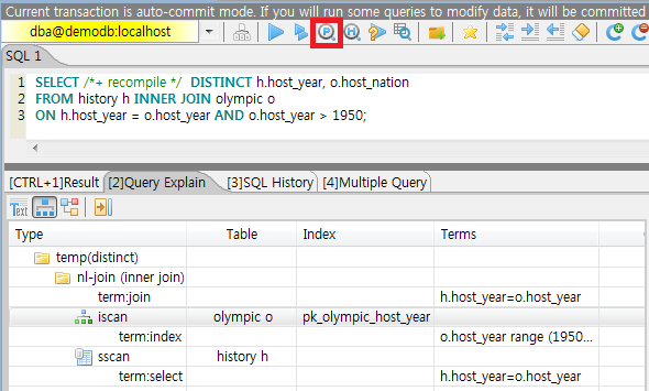
SELECT /*+ recompile */  DISTINCT h.host_year, o.host_nation
FROM history h INNER JOIN olympic o
ON h.host_year = o.host_year AND o.host_year > 1950;

Query plan:

 Sort(distinct)
    Nested-loop join(h.host_year=o.host_year)
        Index scan(olympic o, pk_olympic_host_year, (o.host_year> ?:0 ))
        Sequential scan(history h)

• Sort(distinct): Perform DISTINCT.
• Nested-loop join: Join method is Nested-loop.
• Index scan: Perform index-scan by using pk_olympic_host_year index about olympic table. At that time, the condition which used this index is "o.host_year > ?".

The following shows the result which ran the query after inputting ";plan detail" or "SET OPTIMIZATION LEVEL 513;" in CSQL.

SET OPTIMIZATION LEVEL 513;
--  csql> ;plan detail

SELECT /*+ RECOMPILE */  DISTINCT h.host_year, o.host_nation
FROM history h INNER JOIN olympic o
ON h.host_year = o.host_year AND o.host_year > 1950;

Join graph segments (f indicates final):
seg[0]: [0]
seg[1]: host_year[0] (f)
seg[2]: [1]
seg[3]: host_nation[1] (f)
seg[4]: host_year[1]
Join graph nodes:
node[0]: history h(147/1)
node[1]: olympic o(25/1) (sargs 1)
Join graph equivalence classes:
eqclass[0]: host_year[0] host_year[1]
Join graph edges:
term[0]: h.host_year=o.host_year (sel 0.04) (join term) (mergeable) (inner-join) (indexable host_year[1]) (loc 0)
Join graph terms:
term[1]: o.host_year range (1950 gt_inf max) (sel 0.1) (rank 2) (sarg term) (not-join eligible) (indexable host_year[1]) (loc 0)

Query plan:

temp(distinct)
    subplan: nl-join (inner join)
                 edge:  term[0]
                 outer: iscan
                            class: o node[1]
                            index: pk_olympic_host_year term[1]
                            cost:  1 card 2
                 inner: sscan
                            class: h node[0]
                            sargs: term[0]
                            cost:  1 card 147
                 cost:  3 card 15
    cost:  9 card 15

Query stmt:

select distinct h.host_year, o.host_nation from history h, olympic o where h.host_year=o.host_year and (o.host_year> ?:0 )

On the above output, the information which is related to the query plan is "Query plan:". Query plan is performed sequentially from the inside above line. In other words, "outer: iscan -> inner:scan" is repeatedly performed and at last, "temp(distinct)" is performed. "Join graph segments" is used for checking more information on "Query plan:". For example, "term[0]" in "Query plan:" is represented as "term[0]: h.host_year=o.host_year (sel 0.04) (join term) (mergeable) (inner-join) (indexable host_year[1]) (loc 0)" in "Join graph segments".

The following shows the explanation of the above items of "Query plan:".

• temp(distinct): (distinct) means that CUBRID performs DISTINCT query. temp means that it saves the result to the temporary space.
  • nl-join: "nl-join" means nested loop join.
  • (inner join): join type is "inner join".
    • outer: iscan: performs iscan(index scan) in the outer table.
      • class: o node[1]: It uses o table. For details, see node[1] of "Join graph segments".
      • index: pk_olympic_host_year term[1]: use pk_olympic_host_year index and for details, see term[1] of "Join graph segments".
      • cost: a cost to perform this syntax.
        • card: It means cardinality.
    • inner: sscan: It performs sscan(sequential scan) in the inner table.
      • class: h node[0]: It uses h table. For details, see node[0] of "Join graph segments".
      • sargs: term[0]: sargs represent data filter(WHERE condition which does not use an index); it means that term[0] is the condition used as data filter.
      • cost: A cost to perform this syntax.
        • card: It means cardinality.
  • cost: A cost to perform all syntaxes. It includes the previously performed cost.
    • card: It means cardinality.

Query Plan Related Terms

The following show the meaning for each term which is printed as a query plan.

• Join method: It is printed as "nl-join" on the above. The following are the join methods which are printed on the query plan.
  • nl-join: Nested loop join
  • m-join: Sort merge join
  • idx_join: Nested loop join, and it is a join which uses an index in the inner table as reading rows of the outer table.
• Join type: It is printed as "(inner join)" on the above. The following are the join types which are printed on the query plan.
  • inner join
  • left outer join
  • right outer join: On the query plan, the different "outer" direction with the query's direction can be printed. For example, even if you specified "right outer" on the query, but "left outer" can be printed on the query plan.
  • cross join
• Types of join tables: It is printed as outer or inner on the above. They are separated as outer table and inner table which are based on the position on either side of the loop, on the nested loop join.
  • outer table: The first base table to read when joining.
  • inner table: The target table to read later when joining.
• Scan method: It is printed as iscan or sscan. You can judge that if the query uses index or not.
  • sscan: sequential scan. Also it can be called as full table scan; it scans all of the table without using an index.
  • iscan: index scan. It limits the range to scan by using an index.
• cost: It internally calculate the cost related to CPU, IO etc., mainly the use of resources.
• card: It means cardinality. It is a number of rows which are predicted as selected.

The following is an example of performing m-join(sort merge join) as specifying USE_MERGE hint. In general, sort merge join is used when sorting and merging an outer table and an inner table is judged as having an advantage than performing nested loop join. In most cases, it is desired that you do not perform sort merge join.

SET OPTIMIZATION LEVEL 513;
-- csql> ;plan detail

SELECT /*+ RECOMPILE USE_MERGE*/  DISTINCT h.host_year, o.host_nation
FROM history h LEFT OUTER JOIN olympic o ON h.host_year = o.host_year AND o.host_year > 1950;

Query plan:

temp(distinct)
    subplan: temp
                 order: host_year[0]
                 subplan: m-join (left outer join)
                              edge:  term[0]
                              outer: temp
                                         order: host_year[0]
                                         subplan: sscan
                                                      class: h node[0]
                                                      cost:  1 card 147
                                         cost:  10 card 147
                              inner: temp
                                         order: host_year[1]
                                         subplan: iscan
                                                      class: o node[1]
                                                      index: pk_olympic_host_year term[1]
                                                      cost:  1 card 2
                                         cost:  7 card 2
                              cost:  18 card 147
                 cost:  24 card 147
    cost:  30 card 147

The following performs the idx-join(index join). If performing join by using an index of inner table is judged as having an advantage, you can ensure performing idx-join by specifying USE_IDX hint.

SET OPTIMIZATION LEVEL 513;
-- csql> ;plan detail

CREATE INDEX i_history_host_year ON history(host_year);

SELECT /*+ RECOMPILE */  DISTINCT h.host_year, o.host_nation
FROM history h INNER JOIN olympic o ON h.host_year = o.host_year;

Query plan:

temp(distinct)
    subplan: idx-join (inner join)
                 outer: sscan
                            class: o node[1]
                            cost:  1 card 25
                 inner: iscan
                            class: h node[0]
                            index: i_history_host_year term[0] (covers)
                            cost:  1 card 147
                 cost:  2 card 147
    cost:  9 card 147

On the above query plan, "(covers)" is printed on the "index: i_history_host_year term[0]" of "inner: iscan", it means that Covering Index functionality is applied. In other words, it does not retrieve data storage additionally because there are required data inside the index in inner table.

If you ensure that left table's row number is a lot smaller than the right table's row number on the join tables, you can specify ORDERED hint. Then always the left table will be outer table, and the right table will be inner table.

SELECT /*+ RECOMPILE ORDERED */  DISTINCT h.host_year, o.host_nation
FROM history h INNER JOIN olympic o ON h.host_year = o.host_year;

Query Profiling¶

If the performance analysis of SQL is required, you can use query profiling feature. To use query profiling, specify SQL trace with SET TRACE ON syntax; to print out the profiling result, run SHOW TRACE syntax.

And if you want to always include the query plan when you run SHOW TRACE, you need to add /*+ RECOMPLIE */ hint on the query.

The format of SET TRACE ON syntax is as follows.

SET TRACE {ON | OFF} [OUTPUT {TEXT | JSON}]

• ON: set on SQL trace.
• OFF: set off SQL trace.
• OUTPUT TEXT: print out as a general TEXT format. If you omit OUTPUT clause, TEXT format is specified.
• OUTPUT JSON: print out as a JSON format.

As below, if you run SHOW TRACE syntax, the trace result is shown.

SHOW TRACE;

Below is an example that prints out the query tracing result after setting SQL trace ON.

csql> SET TRACE ON;
csql> SELECT /*+ RECOMPILE */ o.host_year, o.host_nation, o.host_city, n.name, SUM(p.gold), SUM(p.silver), SUM(p.bronze)
        FROM OLYMPIC o, PARTICIPANT p, NATION n
        WHERE o.host_year = p.host_year AND p.nation_code = n.code AND p.gold > 10
        GROUP BY o.host_nation;
csql> SHOW TRACE;

  trace
======================
  '
Query Plan:
  SORT (group by)
    NESTED LOOPS (inner join)
      NESTED LOOPS (inner join)
        TABLE SCAN (o)
        INDEX SCAN (p.fk_participant_host_year) (key range: (o.host_year=p.host_year))
      INDEX SCAN (n.pk_nation_code) (key range: p.nation_code=n.code)

  rewritten query: select o.host_year, o.host_nation, o.host_city, n.[name], sum(p.gold), sum(p.silver), sum(p.bronze) from OLYMPIC o, PARTICIPANT p, NATION n where (o.host_year=p.host_year and p.nation_code=n.code and (p.gold> ?:0 )) group by o.host_nation

Trace Statistics:
  SELECT (time: 1, fetch: 1059, ioread: 2)
    SCAN (table: olympic), (heap time: 0, fetch: 26, ioread: 0, readrows: 25, rows: 25)
      SCAN (index: participant.fk_participant_host_year), (btree time: 1, fetch: 945, ioread: 2, readkeys: 5, filteredkeys: 5, rows: 916) (lookup time: 0, rows: 38)
        SCAN (index: nation.pk_nation_code), (btree time: 0, fetch: 76, ioread: 0, readkeys: 38, filteredkeys: 38, rows: 38) (lookup time: 0, rows: 38)
    GROUPBY (time: 0, sort: true, page: 0, ioread: 0, rows: 5)
'

On the above, later lines of "Trace Statistics:" are the output of the query trace. The following are the items of trace statistics.

SELECT

• time: total estimated time when this query is performed(ms)
• fetch: total page fetching count about this query
• ioread: total I/O read count about this query. disk access count when the data is read

SCAN

• heap: data scanning job without index
  • time, fetch, ioread: the estimated time(ms), page fetching count and I/O read count in the heap of this operation
  • readrows: the number of read rows when this operation is performed
  • rows: the number of result rows when this operation is performed
• btree: index scanning job
  • time, fetch, ioread: the estimated time(ms), page fetching count and I/O read count in the btree of this operation
  • readkeys: the number of the keys which are read in btree when this operation is performed
  • filteredkeys: the number of the keys to which the key filter is applied from the read keys
  • rows: the number of result rows when this operation is performed; the number of result rows to which key filter is applied
• lookup: data accessing job after index scanning
  • time: the estimated time(ms) in this operation
  • rows: the number of the result rows in this operation; the number of result rows to which the data filter is applied

GROUPBY

• time: the estimated time(ms) in this operation
• sort: sorting or not
• page: the number of pages which is read in this operation; the number of used pages except the internal sorting buffer
• rows: the number of the result rows in this operation

The above example can be output as JSON format.

csql> SET TRACE ON OUTPUT JSON;
csql> SELECT n.name, a.name FROM athlete a, nation n WHERE n.code=a.nation_code;
csql> SHOW TRACE;

  trace
======================
  '{
  "Trace Statistics": {
    "SELECT": {
      "time": 29,
      "fetch": 5836,
      "ioread": 3,
      "SCAN": {
        "access": "temp",
        "temp": {
          "time": 5,
          "fetch": 34,
          "ioread": 0,
          "readrows": 6677,
          "rows": 6677
        }
      },
      "MERGELIST": {
        "outer": {
          "SELECT": {
            "time": 0,
            "fetch": 2,
            "ioread": 0,
            "SCAN": {
              "access": "table (nation)",
              "heap": {
                "time": 0,
                "fetch": 1,
                "ioread": 0,
                "readrows": 215,
                "rows": 215
              }
            },
            "ORDERBY": {
              "time": 0,
              "sort": true,
              "page": 21,
              "ioread": 3
            }
          }
        }
      }
    }
  }
}'

On CSQL interpreter, if you use the command to set the SQL trace on automatically, the trace result is printed out automatically after printing the query result even if you do not run SHOW TRACE; syntax.

For how to set the trace on automatically, see Set SQL trace.

Using SQL Hint¶

Using hints can affect the performance of query execution. you can allow the query optimizer to create more efficient execution plan by referring the SQL HINT. The SQL HINTs related tale join, index, and statistics information are provided by CUBRID.

{ CREATE | ALTER } /*+ NO_STATS */ { TABLE | CLASS } ...;

{ CREATE | ALTER | DROP } /*+ NO_STATS */ INDEX ...;

{ SELECT | UPDATE | DELETE } /*+ <hint> [ { <hint> } ... ] */ ...;

MERGE /*+ <merge_statement_hint> [ { <merge_statement_hint> } ... ] */ INTO ...;

<hint> ::=
USE_NL [ (spec_name_comma_list) ] |
USE_IDX [ (spec_name_comma_list) ] |
USE_MERGE [ (spec_name_comma_list) ] |
ORDERED |
USE_DESC_IDX |
NO_DESC_IDX |
NO_COVERING_IDX |
RECOMPILE

<merge_statement_hint> ::=
USE_UPDATE_INDEX (<update_index_list>) |
USE_DELETE_INDEX (<insert_index_list>) |
RECOMPILE

SQL hints are specified by using a plus sign(+) to comments. To use a hint, there are three styles as being introduced on Comment. Therefore, also SQL hint can be used as three styles.

• /*+ hint */
• --+ hint
• //+ hint

The hint comment must appear after the SELECT, CREATE, ALTER, etc. keyword, and the comment must begin with a plus sign (+), following the comment delimiter. When you specify several hints, they are separated by blanks.

The following hints can be specified in CREATE/ALTER TABLE statements and CREATE/ALTER/DROP INDEX statements.

• NO_STATS : Related to a statistical information hint. If it is specified, query optimizer does not update the statistical information after running the DDL statement. Therefore, the DDL performance is improved, but note that the query plan is not optimized.

The following hints can be specified in UPDATE, DELETE and SELECT statements.

• USE_NL : Related to a table join, the query optimizer creates a nested loop join execution plan with this hint.

• USE_MERGE : Related to a table join, the query optimizer creates a sort merge join execution plan with this hint.

• ORDERED : Related to a table join, the query optimizer create a join execution plan with this hint, based on the order of tables specified in the FROM clause. The left table in the FROM clause becomes the outer table; the right one becomes the inner table.

• USE_IDX : Related to an index, the query optimizer creates an index join execution plan corresponding to a specified table with this hint.

• USE_DESC_IDX : This is a hint for the scan in descending index. For more information, see Index Scan in Descending Order.

• NO_DESC_IDX : This is a hint not to use the descending index.

• NO_COVERING_IDX : This is a hint not to use the covering index. For details, see Covering Index.

• NO_STATS : Related to statistics information, the query optimizer does not update statistics information. Query performance for the corresponding queries can be improved; however, query plan is not optimized because the information is not updated.

• RECOMPILE : Recompiles the query execution plan. This hint is used to delete the query execution plan stored in the cache and establish a new query execution plan.

  Note

  If the spec_name is specified together with USE_NL, USE_IDX or USE_MERGE, the specified join method applies only to the spec_name. If USE_NL and USE_MERGE are specified together, the given hint is ignored. In some cases, the query optimizer cannot create a query execution plan based on the given hint. For example, if USE_NL is specified for a right outer join, the query is converted to a left outer join internally, and the join order may not be guaranteed.

MERGE statement can have below hints.

• USE_INSERT_INDEX (<insert_index_list>) : An index hint which is used in INSERT clause of MERGE statement. Lists index names to insert_index_list to use when executing INSERT clause. This hint is applied to <join_condition> of MERGE statement.
• USE_UPDATE_INDEX (<update_index_list>) : An index hint which is used in UPDATE clause of MERGE statement. Lists index names to update_index_list to use when executing UPDATE clause. This hint is applied to <join_condition> and <update_condition> of MERGE statement.
• RECOMPILE : Recompile the query execution plan. Use this hint to remove the old query plan and set the new one to the query plan cache.

The following example shows how to retrieve the years when Sim Kwon Ho won medals and the types of medals. Here, a nested loop join execution plan needs to be created which has the athlete table as an outer table and the game table as an inner table. It can be expressed by the following query. The query optimizer creates a nested loop join execution plan that has the game table as an outer table and the athlete table as an inner table.

SELECT /*+ USE_NL ORDERED  */ a.name, b.host_year, b.medal
FROM athlete a, game b
WHERE a.name = 'Sim Kwon Ho' AND a.code = b.athlete_code;

  name                    host_year  medal
=========================================================
  'Sim Kwon Ho'                2000  'G'
  'Sim Kwon Ho'                1996  'G'

2 rows selected.

The following example shows how to retrieve query execution time with NO_STATS hint to improve the functionality of drop partitioned table (before_2008); any data is not stored in the table. Assuming that there are more than 1 million data in the participant2 table. The execution time in the example depends on system performance and database configuration.

-- without NO_STATS hint
ALTER TABLE participant2 DROP partition before_2008;

Execute OK. (31.684550 sec) Committed.

-- with NO_STATS hint
ALTER /*+ NO_STATS */ TABLE participant2 DROP partition before_2008;

Execute OK. (0.025773 sec) Committed.

Index Hint¶

The index hint syntax allows the query processor to select a proper index by specifying the index in the query. You can specify the index hint by USING INDEX clause or by {USE|FORCE|IGNORE} INDEX syntax after "FROM table" clause.

SELECT ... WHERE ...
[USING INDEX { NONE | [ ALL EXCEPT ] <index_spec> [ {, <index_spec> } ...] } ] [ ; ]

DELETE ... WHERE ...
[USING INDEX { NONE | [ ALL EXCEPT ] <index_spec> [ {, <index_spec> } ...] } ] [ ; ]

UPDATE ... WHERE ...
[USING INDEX { NONE | [ ALL EXCEPT ] <index_spec> [ {, <index_spec> } ...] } ] [ ; ]

<index_spec> ::=
  [table_spec.]index_name [(+) | (-)] |
  table_spec.NONE

FROM table_spec [ <index_hint_clause> ] ...

<index_hint_clause> ::=
  { USE | FORCE | IGNORE } INDEX  ( <index_spec> [, <index_spec>  ...] )

<index_spec> ::=
  [table_spec.]index_name

CREATE TABLE athlete2 (
   code             SMALLINT PRIMARY KEY,
   name             VARCHAR(40) NOT NULL,
   gender           CHAR(1),
   nation_code      CHAR(3),
   event            VARCHAR(30)
);
CREATE UNIQUE INDEX athlete2_idx1 ON athlete2 (code, nation_code);
CREATE INDEX athlete2_idx2 ON athlete2 (gender, nation_code);

SELECT /*+ RECOMPILE */ *
FROM athlete2 USE INDEX (athlete2_idx2)
WHERE gender='M' AND nation_code='USA';

SELECT /*+ RECOMPILE */ *
FROM athlete2
WHERE gender='M' AND nation_code='USA'
USING INDEX athlete2_idx2;

SELECT /*+ RECOMPILE */ *
FROM athlete2 FORCE INDEX (athlete2_idx2)
WHERE gender='M' AND nation_code='USA';

SELECT /*+ RECOMPILE */ *
FROM athlete2
WHERE gender='M' AND nation_code='USA'
USING INDEX athlete2_idx2(+);

SELECT /*+ RECOMPILE */ *
FROM athlete2 IGNORE INDEX (athlete2_idx2)
WHERE gender='M' AND nation_code='USA';

SELECT /*+ RECOMPILE */ *
FROM athlete2
WHERE gender='M' AND nation_code='USA'
USING INDEX athlete2_idx2(-);

SELECT *
FROM athlete2
WHERE gender='M' AND nation_code='USA'
USING INDEX NONE;

SELECT *
FROM athlete2
WHERE gender='M' AND nation_code='USA'
USING INDEX athlete2.NONE;

SELECT *
FROM athlete2
WHERE gender='M' AND nation_code='USA'
USING INDEX ALL EXCEPT athlete2_idx2;

SELECT *
FROM athlete2 USE INDEX (athlete2_idx2, athlete2_idx1)
WHERE gender='M' AND nation_code='USA';

SELECT *
FROM athlete2
WHERE gender='M' AND nation_code='USA'
USING INDEX athlete2_idx2, athlete2_idx1;

SELECT *
FROM tab1, tab2
WHERE ...
USING INDEX tab1.idx1, tab2.NONE;

SELECT ...
FROM tab1, tab2 USE INDEX(tab1.idx1)
WHERE ... ;

SELECT ...
FROM tab1, tab2
WHERE ...
USING INDEX tab1.idx1;

Optimization using indexes¶

CREATE TABLE t (col1 INT, col2 INT, col3 INT);
CREATE INDEX i_t_col1_col2_col3 ON t (col1,col2,col3);
INSERT INTO t VALUES (1,2,3),(4,5,6),(10,8,9);

-- csql> ;plan simple
SELECT * FROM t WHERE col1 < 6;

Query plan:
 Index scan(t t, i_t_col1_col2_col3, [(t.col1 range (min inf_lt t.col3))] (covers))

         col1         col2         col3
=======================================
            1            2            3
            4            5            6

CREATE TABLE tab(c VARCHAR(32));
INSERT INTO tab VALUES('abcd'),('abcd    '),('abcd ');
CREATE INDEX i_tab_c ON tab(c);

-- csql>;plan simple
SELECT * FROM tab WHERE c='abcd    ' USING INDEX i_tab_c(+);

Query plan:
 Index scan(tab tab, i_tab_c, (tab.c='abcd    ') (covers))

 c
======================
'abcd'
'abcd'
'abcd'

SELECT * FROM tab WHERE c='abcd    ' USING INDEX tab.NONE;

Query plan:
 Sequential scan(tab tab)

 c
======================
'abcd'
'abcd    '
'abcd '

SELECT *
FROM tab
WHERE col1 > 0
ORDER BY col1, col2

SELECT *
FROM tab
WHERE col2=val
ORDER BY col1,col3;

CREATE TABLE tab (i INT, j INT, k INT);
CREATE INDEX i_tab_j_k on tab (j,k);
INSERT INTO tab VALUES (1,2,3),(6,4,2),(3,4,1),(5,2,1),(1,5,5),(2,6,6),(3,5,4);

SELECT i,j,k
FROM tab
WHERE j > 0
ORDER BY j,k;

--  the  selection from the query plan dump shows that the ordering index i_tab_j_k was used and sorting was not necessary
--  (/* --> skip ORDER BY */)
Query plan:
iscan
    class: tab node[0]
    index: i_tab_j_k term[0]
    sort:  2 asc, 3 asc
    cost:  1 card 0
Query stmt:
select tab.i, tab.j, tab.k from tab tab where ((tab.j> ?:0 )) order by 2, 3
/* ---> skip ORDER BY */

            i            j            k
=======================================
            5            2            1
            1            2            3
            3            4            1
            6            4            2
            3            5            4
            1            5            5
            2            6            6

SELECT /*+ RECOMPILE */ j,k
FROM tab
WHERE j > 0
ORDER BY j,k;

--  in this case the index i_tab_j_k is a covering index and also respects the ordering index property.
--  Therefore, it is used as a covering index and sorting is not performed.

Query plan:
iscan
    class: tab node[0]
    index: i_tab_j_k term[0] (covers)
    sort:  1 asc, 2 asc
    cost:  1 card 0

Query stmt: select tab.j, tab.k from tab tab where ((tab.j> ?:0 )) order by 1, 2
/* ---> skip ORDER BY */

            j            k
==========================
            2            1
            2            3
            4            1
            4            2
            5            4
            5            5
            6            6

CREATE INDEX i_tab_j_k ON tab (i,j,k);
SELECT /*+ RECOMPILE */ i,j,k
FROM tab
WHERE i > 0
ORDER BY j,k;

-- since an index on (i,j,k) is now available, it will be used as covering index. However, sorting the results according to
-- the ORDER BY  clause is needed.
Query plan:
temp(order by)
    subplan: iscan
                 class: tab node[0]
                 index: i_tab_i_j_k term[0] (covers)
                 sort:  1 asc, 2 asc, 3 asc
                 cost:  1 card 1
    sort:  2 asc, 3 asc
    cost:  7 card 1

Query stmt: select tab.i, tab.j, tab.k from tab tab where ((tab.i> ?:0 )) order by 2, 3

            i            j            k
=======================================
            5            2            1
            1            2            3
            3            4            1
            6            4            2
            3            5            4
            1            5            5
            2            6            6

SELECT *
FROM tab
[WHERE ...]
ORDER BY a DESC

CREATE TABLE di (i INT);
CREATE INDEX i_di_i on di (i);
INSERT INTO di VALUES (5),(3),(1),(4),(3),(5),(2),(5);

-- The query will be executed with an ascending scan.

SELECT  *
FROM di
WHERE i > 0
LIMIT 3;

Query plan:

Index scan(di di, i_di_i, (di.i range (0 gt_inf max) and inst_num() range (min inf_le 3)) (covers))

            i
=============
            1
            2
            3

-- We now run the following query, using the ''use_desc_idx'' SQL hint:

SELECT /*+ USE_DESC_IDX */ *
FROM di
WHERE i > 0
LIMIT 3;

Query plan:
 Index scan(di di, i_di_i, (di.i range (0 gt_inf max) and inst_num() range (min inf_le 3)) (covers) (desc_index))

            i
=============
            5
            5
            5

-- We also run the same query, this time asking that the results are displayed in descending order.
-- However, no hint is given.
-- Since ORDER BY...DESC clause exists, CUBRID will use descending scan, even though the hint is not given,
-- thus avoiding to sort the records.

SELECT *
FROM di
WHERE i > 0
ORDER BY i DESC LIMIT 3;

Query plan:
 Index scan(di di, i_di_i, (di.i range (0 gt_inf max)) (covers) (desc_index))

            i
=============
            5
            5
            5

SELECT *
FROM tab
WHERE col1 > 0
GROUP BY col1,col2

SELECT *
FROM tab
WHERE col2=val
GROUP BY col1,col3

CREATE INDEX i_T_a_b_c ON T(a, b, c);
SELECT a, MIN(b), c, MAX(b) FROM T WHERE a > 18 GROUP BY a, b;

CREATE TABLE tab (i INT, j INT, k INT);
CREATE INDEX i_tab_j_k ON tab (j, k);
INSERT INTO tab VALUES (1,2,3),(6,4,2),(3,4,1),(5,2,1),(1,5,5),(2,6,6),(3,5,4);

SELECT i,j,k
FROM tab
WHERE j > 0
GROUP BY j,k;

--  the  selection from the query plan dump shows that the index i_tab_j_k was used and sorting was not necessary
--  (/* ---> skip GROUP BY */)

Query plan:
iscan
    class: tab node[0]
    index: i_tab_j_k term[0]
    sort:  2 asc, 3 asc
    cost:  1 card 0

Query stmt:
select tab.i, tab.j, tab.k from tab tab where ((tab.j> ?:0 )) group by tab.j, tab.k
/* ---> skip GROUP BY */
            i            j            k
            5            2            1
            1            2            3
            3            4            1
            6            4            2
            3            5            4
            1            5            5
            2            6            6

ALTER TABLE tab CHANGE COLUMN j j INT NOT NULL;

SELECT *
FROM tab
GROUP BY j,k;

--  the  selection from the query plan dump shows that the index i_tab_j_k was used (since j has the NOT NULL constraint )
--  and sorting was not necessary (/* ---> skip GROUP BY */)
Query plan:
iscan
    class: tab node[0]
    index: i_tab_j_k
    sort:  2 asc, 3 asc
    cost:  1 card 0

Query stmt: select tab.i, tab.j, tab.k from tab tab group by tab.j, tab.k
/* ---> skip GROUP BY */
=== <Result of SELECT Command in Line 1> ===
            i            j            k
=======================================
            5            2            1
            1            2            3
            3            4            1
            6            4            2
            3            5            4
            1            5            5
            2            6            6